Virtual Chess Rook
The Virtual Chess Rook is a simulated robot (virtual) that moves north, south, east, and west on a grid just like a Chess Rook! It will be explained better later.
This project is a result of the Junior Scientific Research Program (Iniciação Científica in portuguese) made by Henrique Ferreira Jr. and advised by Ph.D. Daniel R. Figueiredo. The objective here is to use a simple robot and environment models to perform many simulations efficiently. Then, with these simulations results we do the analyses and propose new methods.
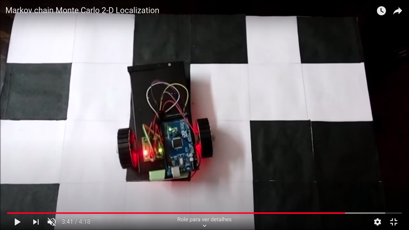
Is important to say that this model was inspired in the video bellow:
Overview
This project relies on Monte Carlo Localization algorithm as the name The Monte Carlo Robots suggests. Thus, the analyses made here focus on evaluating it's localization performance under different scenes. Let's starting talking about the robot and environment models used here (also explained in the papers).
Environment model
We consider an environment in the form of a squared two-dimensional grid
with wrap-around (i.e., torus) of size (n, n). That is, each location in
the environment has exactly four neighboring locations and moving exactly
n + 1 steps in the same direction returns to the starting point. Each
location in the environment corresponds to a possible location for the
robot, which in this case has n^2 different locations. Exactly p
landmarks are added to the environment, all identical (this means that the
robot knows it is in a location that has a landmark, but not what is this
location.
Robot model
Initially, in time t = 0, the robot is positioned randomly and uniformly
in some state of the environment and it does not have any information
about its position.
We will consider a discrete-time model, where at each step the robot may perform a movement or a reading to identify the presence of a reference point. The move moves the robot to an adjacent location: up, down, left, or right.
To model the noise in the robot motion, we will consider that the
robot has a chance of overshooting p_overshoot, i.e. moving an additional
position in the same chosen direction, and a chance of undershooting
p_undershoot, i.e., staying in the same location (not moving). Thus, the
chance of do the exact motion is p_exact = 1 - p_overshoot - p_undershoot.
It is important to note that the robot is not able to determine if there has been an overshoot or
undershoot when moving.
To model the noise in the identification of reference points, a reading
tells the robot whether the current location is has a landmark or does not
have a landmark with the same chance of error p_miss. That is, the robot
correctly detects the presence or absence of a landmark in its location
with p_hit = 1 - p_miss chance.

The image above illustrates an environment where n = 10 and p = 50.
The presence of a reference point is denoted by a black square and the
absence by a white square. For a robot in the red square the blue squares
shows the possibles next location after a movement.
Documentation Roadmap
This documentation is divided in two parts:
- High level documentation: With the projects decisions, reflections, and history. Will not focus on the discussion already in the articles.
- Code documentation: Implementation details of the classes used in this project.
So the roadmap is this way:
- Home: This page.
- Project Documentation
- First Version: A little of history about previous versions before the first article.
- ENIAC 2018: The changes to make this article.
- Code Optimization: Smart chances to reduce 80% of the computational time in the code.
- Variants: Other analyses like, map with border or finding the worst map...
- ENIAC 2019: The changes to make this article.
- CTIC 2020: The changes to make this article.
- Code Documentation
- map.py: The bi-dimensional grid map implementation for Monte Carlo Localization.
- simulator.py: The robot model simulator. It simulates the robot position, movements and sensor readings.
- mcl.py: The Monte Carlo Localization algorithm implementation. Inherits the Simulator.
- simulated-annealing.py: The implementation of the Simulated Annealing algorithm using the Boltzmann Distribution.